12-01 · Meaningful estimates: one figure, one paragraph

Start here

Four groups of three; rotate driver, outcome translator and uncertainty auditor. Essential teaching takes place in class; no new pre-class reading is required. Open the instructor-supplied 12-estimation-communication Posit Cloud project; its complete student files are already in the project root.

Teaching slides Workshop slides

Worksheet · Recap · Data dictionary

Run estimates-student.R from the student project root. Required packages: lme4, performance, marginaleffects and ggplot2. The script and its supplied references analyse only a separate, invented cress germination example. They do not choose an analysis or answer for an assessed project. The code below uses website-relative paths; the student script uses data/cress-trays.csv from its own root.

Opening recall — 12:30–12:45

Recall the calf study: researchers assign one diet to each calf and weigh it five times. Why do five weights from the same calf belong together? What would change if researchers assigned diet to whole pens instead? Then explain what researchers do in your own project: name the animals or groups they treat or follow, the measurements they record, and the comparison you want to make.

Essential teaching — 12:45–13:15

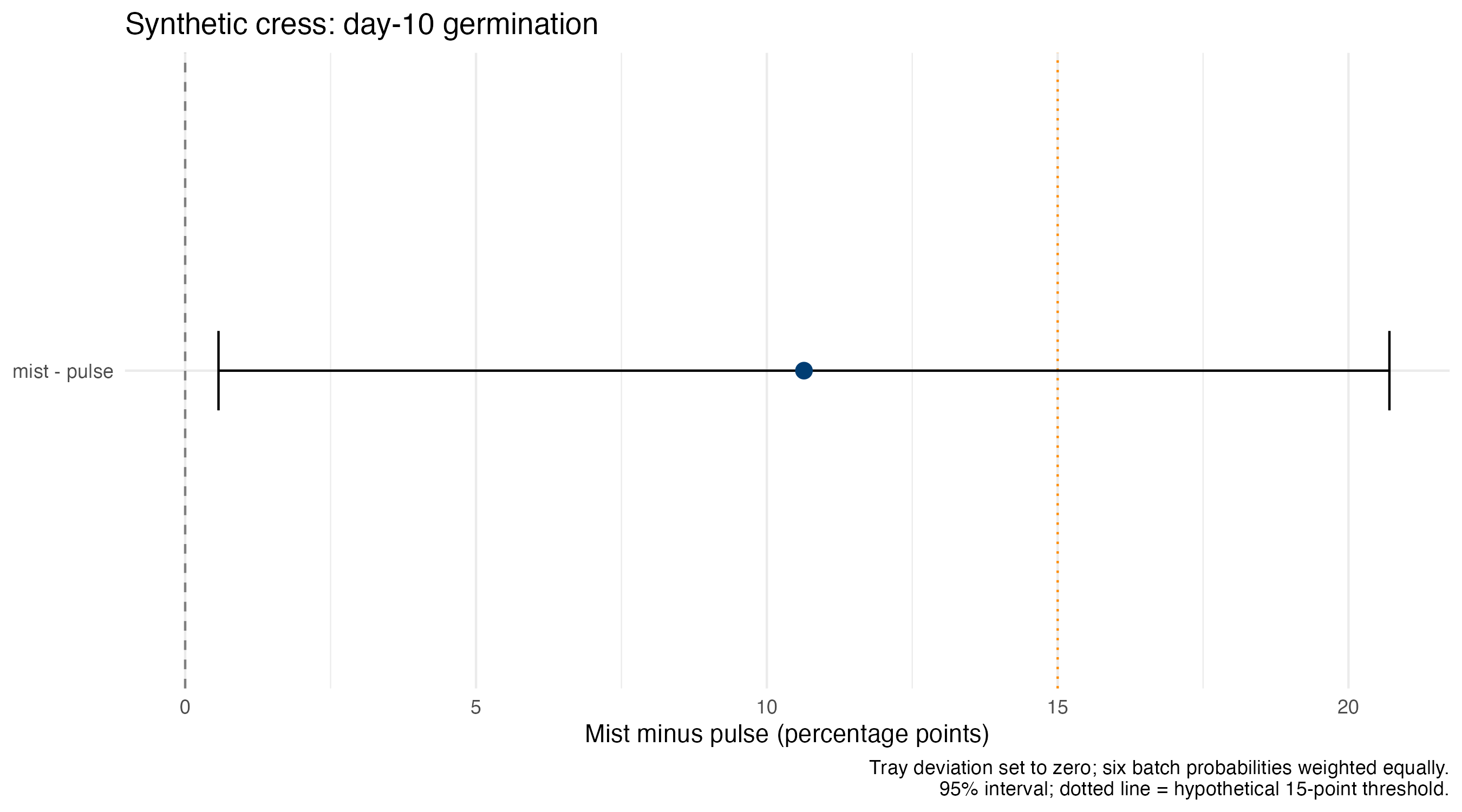
Before fitting, say what would answer the study question. For the cress example below, compare the chance of sprouting with mist and pulse watering on day 10, give each sowing batch equal weight, and set the shared tray difference to zero. We will express the difference in percentage points and distinguish uncertainty in that estimate from variation in seed outcomes.

A distinct invented study

Researchers sow 25 cress seeds in each of 48 trays, in six batches. Within each batch, they randomly choose four trays for pulse watering and four for mist watering. On day 10 they count how many seeds have sprouted in each tray. They assign watering to 24 trays per method; all 25 seeds in a tray share that method. These are invented observations and study details, not evidence about growing cress.

Read the counts

library("dplyr")

library("lme4")
library("performance")
library("marginaleffects", warn.conflicts = FALSE)
trays <- readr::read_csv("../assets/week-12/data/cress-trays.csv")
trays <- trays |>
  mutate(
    watering = factor(watering, levels = c("pulse", "mist")),
    batch = factor(batch),
    tray_id = factor(tray_id)
  )
head(trays |> select("tray_id", "watering", "seeds_sown", "seeds_sprouted"), 3)

# A tibble: 3 × 4
  tray_id watering seeds_sown seeds_sprouted
  <fct>   <fct>         <dbl>          <dbl>
1 T01     mist             25             11
2 T02     mist             25             17
3 T03     mist             25             12

One row is one tray. Pulse is the reference watering condition.

Step 2: fit the tray count model

Each tray can have its own tendency to sprout, around the watering and batch pattern.

fit <- glmer(
  cbind(seeds_sprouted, seeds_sown - seeds_sprouted) ~
    watering + batch + (1 | tray_id),
  data = trays,
  family = binomial()
)
summary(fit)

Generalized linear mixed model fit by maximum likelihood (Laplace
  Approximation) [glmerMod]
 Family: binomial  ( logit )
Formula: cbind(seeds_sprouted, seeds_sown - seeds_sprouted) ~ watering +  
    batch + (1 | tray_id)
   Data: trays

      AIC       BIC    logLik -2*log(L)  df.resid 
    287.6     302.6    -135.8     271.6        40 

Scaled residuals: 
     Min       1Q   Median       3Q      Max 
-1.43101 -0.29504 -0.05139  0.49570  1.04567 

Random effects:
 Groups  Name        Variance Std.Dev.
 tray_id (Intercept) 0.3581   0.5984  
Number of obs: 48, groups:  tray_id, 48

Fixed effects:
              Estimate Std. Error z value Pr(>|z|)  
(Intercept)  -0.477441   0.279414  -1.709   0.0875 .
wateringmist  0.435295   0.211707   2.056   0.0398 *
batchB2       0.068796   0.364614   0.189   0.8503  
batchB3       0.435833   0.365244   1.193   0.2328  
batchB4       0.001746   0.365056   0.005   0.9962  
batchB5       0.057323   0.367629   0.156   0.8761  
batchB6       0.726784   0.366622   1.982   0.0474 *
---
Signif. codes:  0 '***' 0.001 '**' 0.01 '*' 0.05 '.' 0.1 ' ' 1

Correlation of Fixed Effects:
            (Intr) wtrngm btchB2 btchB3 btchB4 btchB5
wateringmst -0.384                                   
batchB2     -0.654  0.002                            
batchB3     -0.654  0.005  0.500                     
batchB4     -0.654  0.004  0.500  0.499              
batchB5     -0.646 -0.006  0.497  0.495  0.496       
batchB6     -0.655  0.013  0.498  0.498  0.497  0.493

VarCorr(fit)

 Groups  Name        Std.Dev.
 tray_id (Intercept) 0.59837

The binomial model describes sprouts out of 25 seeds. (1 | tray_id) allows a shared tray difference, called a random intercept. The coefficient compares log-odds, not probabilities: odds are the chance of sprouting divided by the chance of not sprouting.

Check the count model

set.seed(1212)
check_overdispersion(fit)

# Overdispersion test (using simulated residuals)

 dispersion ratio = 1.203
          p-value = 0.168

No overdispersion detected.

check_singularity(fit)

[1] FALSE

Do counts vary more than the fitted model expects? Has the estimated tray variation collapsed to zero?

These checks do not establish that every model assumption is correct.

Step 3: say which probabilities we want

Trays can have higher or lower chances of sprouting than their watering-and-batch pattern predicts. We call this a tray deviation. Set it to zero, predict the chance in each batch, then average the six probabilities equally.

grid <- tidyr::crossing(
  watering = trays$watering,
  batch = trays$batch
) |>
  mutate(tray_id = trays$tray_id[1])
probabilities <- avg_predictions(
  fit,
  newdata = grid,
  by = "watering",
  type = "response",
  re.form = NA
)
probabilities


 watering Estimate Std. Error    z Pr(>|z|)     S 2.5 % 97.5 %
    pulse    0.436     0.0362 12.0   <0.001 108.6 0.365  0.506
    mist     0.542     0.0365 14.9   <0.001 163.7 0.471  0.613

Type: response

type = "response" asks for probabilities; re.form = NA leaves out the fitted tray differences. Zero means no additional tray departure, not zero sprouts. We do not average over trays whose departures vary.

Step 4: mist minus pulse

library("dplyr")

difference <- avg_comparisons(
  fit,
  newdata = grid,
  variables = list(watering = c("pulse", "mist")),
  type = "response",
  re.form = NA
)
print(difference)


 Estimate Std. Error    z Pr(>|z|)   S   2.5 % 97.5 %
    0.106     0.0514 2.07   0.0383 4.7 0.00573  0.207

Term: watering
Type: response
Comparison: mist - pulse

# Express the same estimate and interval in percentage points for the figure.
comparison <- as.data.frame(difference)
comparison <- comparison |>
  mutate(across(c(estimate, std.error, conf.low, conf.high), ~ 100 * .x))
comparison

      term     contrast estimate std.error statistic    p.value  s.value
1 watering mist - pulse 10.63834  5.135468  2.071542 0.03830816 4.706205
   conf.low conf.high
1 0.5730062  20.70367

Percentage points, with an approximate 95% interval. Second condition minus first.

An interval for a probability or contrast does not contain 95% of seeds or trays. A seed outcome is binary; future tray counts also vary because of their tray environment and binomial sampling. Confidence coverage is a repeated-sampling property under assumptions, not a 95% probability assigned to a fixed true effect in this observed interval.

Meaningful-outcomes activity — 13:15–13:40

Use the teaching data and worksheet. Explain how researchers assigned watering to trays, why each count is out of 25, how the shared tray term represents growing conditions, and which probabilities we compare. Read the printed output or teaching contrast table, probabilities and model output if computing is unavailable.

Report magnitude, direction, units and interval; compare a hypothetical worthwhile change chosen before seeing results of 15 percentage points, explicitly an invented classroom value. An interval excluding zero can still span that threshold. For separate hypothetical probabilities .40 and .55, calculate the percentage-point difference, ratio and relative change. Those illustrative values are not this model’s fitted results.

Break 13:40–13:55.

One figure, one paragraph — 13:55–14:30

Using the teaching contrast figure, make or annotate one figure and write 100–150 words. State the watering question, how researchers assigned trays and counted sprouts, the model and estimated difference, its interval, practical meaning and one limitation. In the caption name the comparison, units, day 10, equal batch weights, tray difference set to zero, interval and invented data. This is communication practice on the separate teaching example.

Peer review — 14:30–14:55

Swap teaching-example drafts. Recover the question and conclusion unaided; check direction, units, population/time, interval, allocation and causal wording. Give one change that improves the scientific explanation and one feature to preserve. Revise immediately.

Break 14:55–15:10.

Your project workshop — 15:10–15:45

Use your own approved data or raw fallback. State what researchers do to the animals or groups, what they measure, and which comparison answers your question. Propose a model for those records and checks of its assumptions. Explain which animals or groups your estimate concerns, what you hold fixed or average over, and one alternative assumption worth comparing. The teaching script is not a project analysis recipe. Ask the instructor about a decision needing clarification; record your next action. Existing information and in-class consultation should support your choices without a supplied fitted answer.