11-01 · Fit, predict and check change through time
Start here
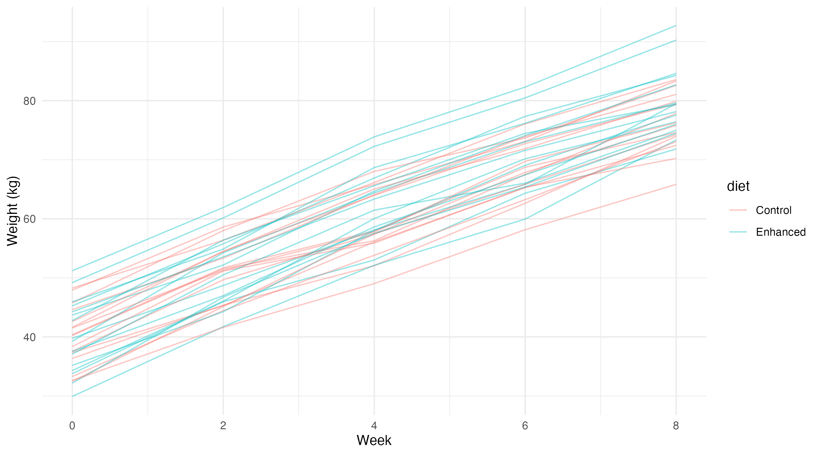
Researchers assign Control or Enhanced feed to each of 32 calves, balancing the two diets within each of four rooms. They weigh each calf at weeks 0, 2, 4, 6 and 8. These invented records are the same as in Class 10. We want to describe growth and compare expected calf weights at week 8.
Work in four groups of three. One person runs the code, one explains the output, and one checks that the analysis matches what researchers did. Rotate roles after the breaks. No new preparation is required.
Open the instructor-supplied Posit Cloud project for 11-longitudinal-data, open week-11.Rproj, and run longitudinal-student.R one section at a time. Run setup.R if packages are missing. The examples use lme4 for fitting, performance for checks, marginaleffects for expected weights and differences, and ggplot2 for plots.
Each calf keeps one diet for eight weeks. Researchers record week 0 before feeding starts. How many calves receive each diet? Why does weighing a calf five times help us describe its growth without adding another calf to the diet comparison?
In Class 10, treating visits as named groups allowed a separate mean at every visit. What restriction would a straight growth line add? How does (1 | calf) allow some calves to remain heavier than others? Contrast this study with the crossover example, where researchers give the same animal both treatments in a planned order.
Growth lines and curves — 08:15–08:45
A calf’s sequence of weights describes its growth path, also called its trajectory. Compare a straight line with a curve that allows growth to slow. Keep the same diet groups, rooms and calf grouping in both models. A difference in diet growth rates is called a diet-by-time interaction.
The week-0 diet coefficient allows the two groups to differ before feeding begins. It therefore describes chance starting differences. To compare expected weights at week 8, combine the starting difference with the diet difference in growth over eight weeks. The workshop code below asks marginaleffects to make this comparison directly.
Growth-story cards — 08:45–09:10
Each group receives one card. Sketch the weights described, suggest a line or curve, and explain why two weights from the same calf might remain related. For the illness card, state what researchers need to find out about missed weighings. Swap explanations with another group. The cards describe hypothetical studies; there are no extra datasets to fit.
Break 09:10–09:25.
Fit, predict and check — 09:25–10:25
Read the records
calf identifies the animal and room its room. weight_kg is the recorded weight. The script creates week from time_week. Treat diet, calf and room as named groups using factor().
# A tibble: 3 × 4
  calf  diet     week weight_kg
  <fct> <fct>   <dbl>     <dbl>
1 C01   Control     0      47.9
2 C01   Control     2      58.6
3 C01   Control     4      65.8
Fit two growth descriptions
diet * week allows different starting weights and growth rates for the two diets. (1 | calf) adds a shared calf difference, called a random intercept. I(week^2) bends both diet paths by the same amount. Rooms stay in both models because researchers assigned both diets within every room.
AIC compares how well each model fits after allowing for extra model terms; a smaller value is better on that comparison. It does not prove that a model describes every feature of the study. The AIC table uses explicit maximum-likelihood copies (REML = FALSE) of both models on the same observations. Keep the REML fits for estimation; REML likelihoods must not be compared across different fixed effects.
Ask what the checks examine
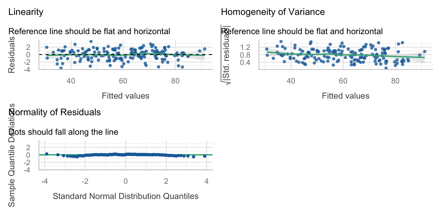
The first check asks whether the estimated spread of calf differences is nearly zero. The second examines whether the remaining errors have the bell-shaped distribution assumed by the model. An error is the observed weight minus the fitted weight; it is also called a residual.
check_singularity(curved)
[1] FALSE
check_normality(curved)
OK: residuals appear as normally distributed (p = 0.268).
FALSE in the first result means the estimated calf spread is not nearly zero. Neither result proves that errors from nearby visits are unrelated.
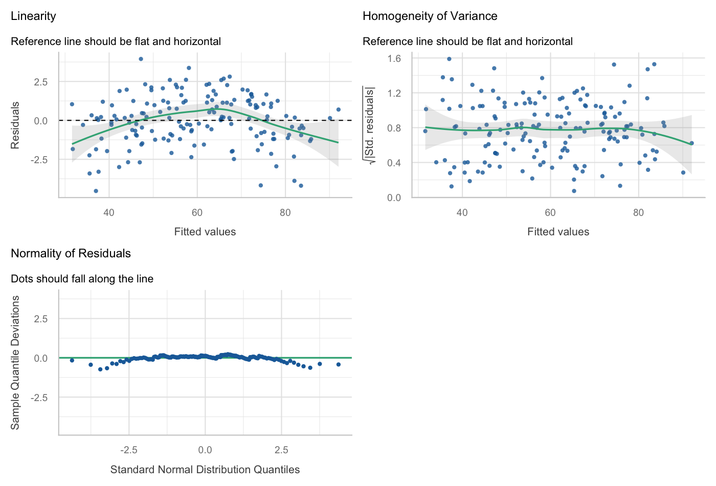
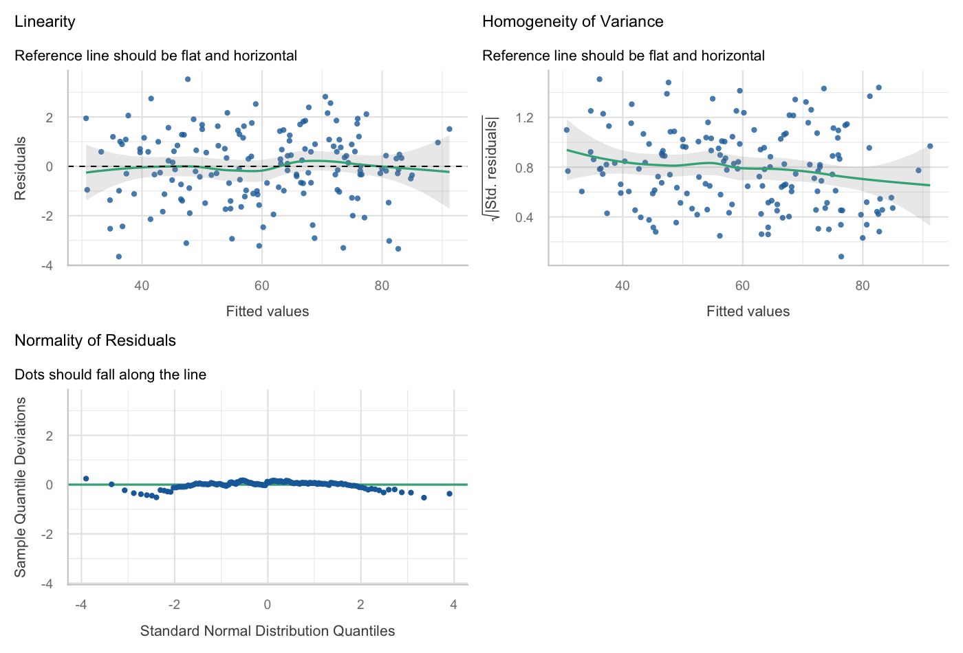
The panels examine error shape, missed patterns and changing error spread. Explain each axis before deciding what the plot suggests.
Check the growth pattern
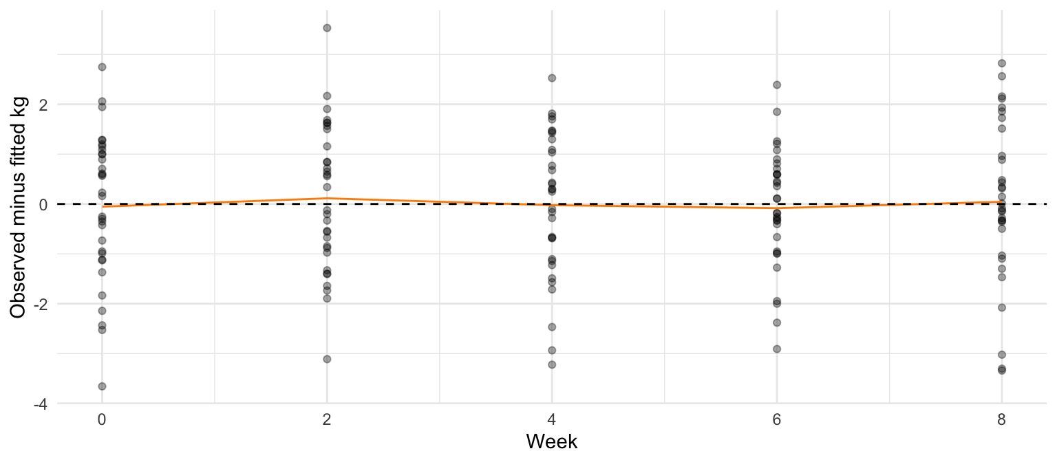
We also need a plot specific to the calf question: are errors systematically positive or negative at particular weeks? The orange line joins the mean error at each visit.
library("dplyr")d <- d |>mutate(error_kg =residuals(curved, type ="response") )ggplot(d, aes(week, error_kg)) +geom_point(alpha = .35) +stat_summary(fun = mean, geom ="line", colour ="darkorange") +geom_hline(yintercept =0, linetype =2) +labs(x ="Week", y ="Observed minus fitted kg") +theme_minimal()
Does this line still bend with time? A better average growth curve can leave errors from the same calf related.
Say which calves and rooms the question concerns
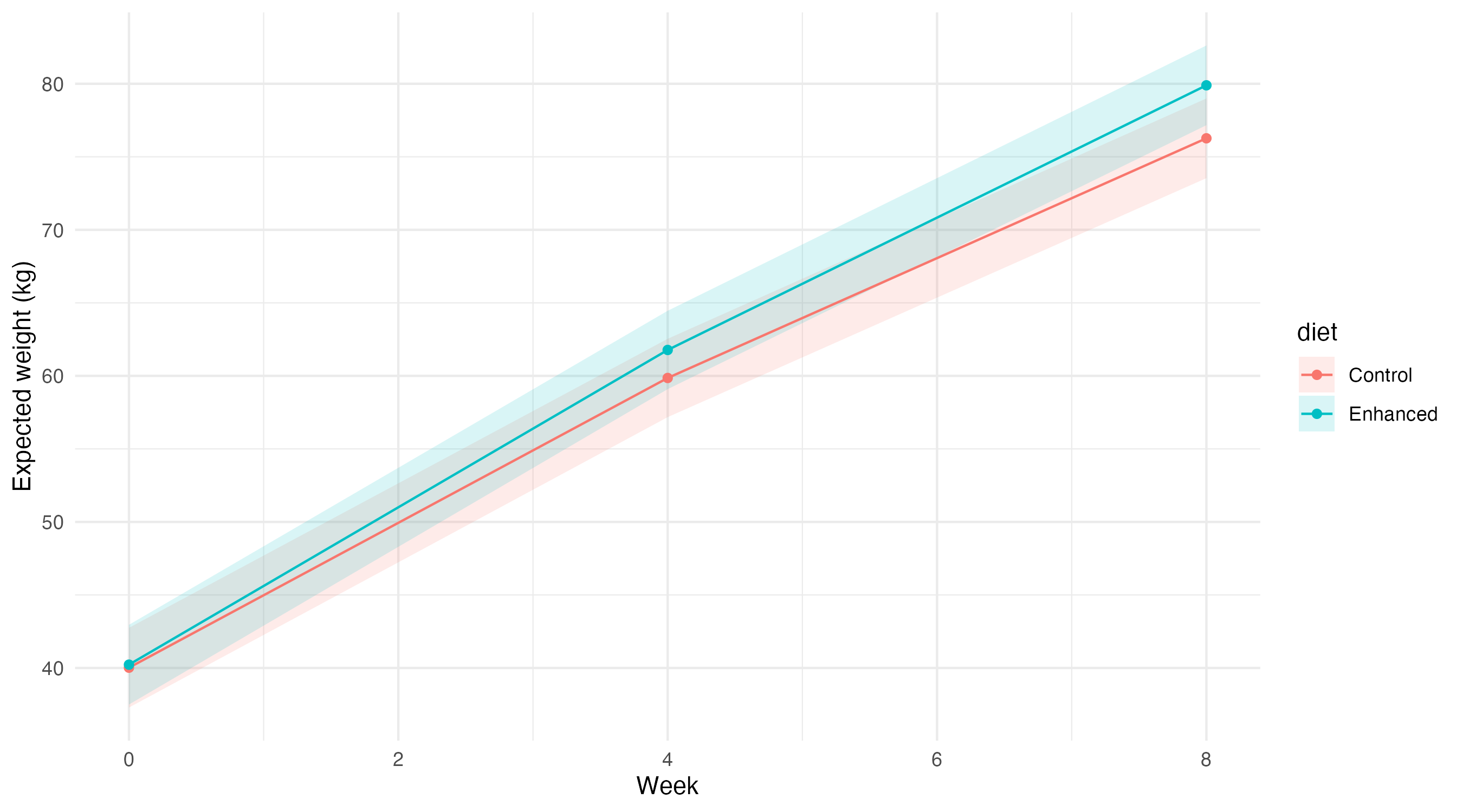
We want expected weights for new calves at weeks 0, 4 and 8, giving each room equal weight. Create every combination of diet, week and room once. The calf ID makes a valid record for prediction; re.form = NA below leaves out that animal’s fitted difference.
Weights and interval limits are in kg. These intervals describe uncertainty in expected weights, rather than the spread of individual calves.
Compare Enhanced minus Control
At each week, compare expected Enhanced and Control weights with the same equal room weighting. The first condition in variables is subtracted from the second.
Read the week-8 estimate and both ends of its approximate 95% interval. The week-0 row describes starting differences before feeding; it is not a diet effect already received.
Interpret the optional visit-correlation example
A calf may weigh more than the model predicts at one visit and again at the next. That is a possible relationship between its remaining errors. The supplied extension keeps the same mean growth curve and calf difference while allowing this additional relationship to weaken as visits get further apart. Its technical name is AR(1).
Read the extension output. The estimated correlation concerns errors two weeks apart after allowing for the mean and shared calf difference; it is not the correlation between raw weights. Fitting this extension is optional. Do not choose the model according to whether its diet interval crosses zero.
Retrieve your project brief, saved Class 10 plan and data. Name the animals or groups researchers treated or followed, and what they measured. Explain why your outcome needs a continuous, yes/no or count model, and how the model connects measurements from the same animal or group.
Fit your proposed preliminary model, inspect its checks and trace one useful estimate to your question. Record a concern and an alternative worth comparing because of the study design or biology. Explain any change from your saved plan. Your project may have no repeated measurements; do not add calf time terms to a pen or yes/no study without a reason.
Groups with data-access problems use the supplied raw-data fallback. If code fails, keep your study description, proposed analysis and descriptive plot, and record the specific calculation that needs support.
Reports and exit — 11:15–11:30
Each group gives one preliminary result and one unresolved concern in 90 seconds. Individually explain why five weighings of each of 32 calves do not create 160 calves receiving a diet. Name an assumption that still needs checking after adding a curved growth path.
Save your morning project work for the afternoon workshop. Use the optional consolidation as needed when revising your draft before 25 November.