Use lme4, performance and marginaleffects directly to analyse repeated calf weights and a cow crossover.
Start here
Work in four seated groups of three. Open the instructor-supplied Posit Cloud project 10-repeated-measures, then week-10.Rproj. Run setup.R once if packages are missing. Open in-class-student.R and run its sections in order from the project root. It shows the package calls directly; there is no analysis helper to source.
The driver runs code, the explainer interprets output, and the design checker checks assignments and units. Rotate after the first break. If computing fails, use the supplied reference results and keep explaining the design and output.
Both datasets are synthetic teaching examples. Numerical results are practice in reasoning, not empirical feeding advice.
Opening recall — 12:30–12:40
The previous example assigned diet to pens. Today’s calf example assigns diet separately to individually housed calves, within rooms. Explain why these studies have different numbers of animals or pens to which researchers assigned diets. Repeated weights help describe change, but do not create additional diet assignments.
Calves: one diet, five weights — 12:40–13:15
There are 32 calves in four rooms. Within each room, four calves receive Control and four Enhanced. Diets start after the baseline measurement, followed by weights at weeks 2, 4, 6 and 8. Our first question is: how much heavier are Enhanced calves on average at week 8?
Read the data, declare the categories and check the allocation count. factor() marks a column as a category; distinct() keeps each calf’s allocation once.
# A tibble: 3 × 6
  room  calf  diet    time_week weight_kg time_factor
  <fct> <fct> <fct>       <dbl>     <dbl> <fct>
1 R1    C01   Control         0      47.9 0
2 R1    C01   Control         2      58.6 2
3 R1    C01   Control         4      65.8 4
d |>distinct(calf, room, diet) |>count(room, diet)
# A tibble: 8 × 3
  room  diet         n
  <fct> <fct>    <int>
1 R1    Control      4
2 R1    Enhanced     4
3 R2    Control      4
4 R2    Enhanced     4
5 R3    Control      4
6 R3    Enhanced     4
7 R4    Control      4
8 R4    Enhanced     4
Fit a model that allows rooms to have different average weights, the diet gap to change between visits, and calves to have persistent differences. lmer() assumes roughly bell-shaped unexplained differences. REML = TRUE estimates group and residual variation while allowing for the fixed effects.
avg_comparisons() estimates Enhanced minus Control in kg, separately at each week. re.form = NA leaves out each calf’s fitted weight difference from the usual weight. The complete, balanced room allocation gives equal room representation here. The intervals are approximate 95% intervals for the mean comparison under the specified model, not ranges for individual weights.
The first check returns TRUE when the fitting calculation succeeds. The second returns FALSE when estimated variation in calves’ usual weights has not collapsed to zero. Neither establishes that nearby weights have no further shared influence. Give the week-8 estimate, its interval and this remaining limitation. Explain why a baseline gap cannot be a consequence of diets that have not yet started.
Design a crossover — 13:15–13:40
In the cow example, each animal receives both rations. This is called a crossover. Twenty-four cows are randomly assigned to order AB or BA, twelve per order. The assigned order is called the sequence. Each cow has a first and a second treatment period. The outcome is average daily intake over the final three days of each ten-day treatment period.
A ten-day treatment-free gap is specified between periods. A washout gives earlier treatment effects time to wear off. Carryover means they remain. Ten days is a teaching assumption, not a recommendation. A real study needs evidence about the particular ration and outcome.
Use the design cards. Explain why all cows receiving A then B would mix up treatment with a general period change. Decide whether crossover is suitable for reversible intake effects, vaccines with lasting effects, and irreversible growth. Identify the evidence needed to justify the gap. Adding a sequence term to a model cannot create washout.
Break 13:40–13:55.
Fit the cow comparison — 13:55–14:55
Read the records and retain cow, assigned order and scheduled period. Each row represents one cow in one treatment period, not a daily reading and not a new animal newly assigned a treatment.
# A tibble: 4 × 5
  cow   sequence period treatment intake_kg_day
  <fct> <fct>    <fct>  <fct>             <dbl>
1 W01   AB       1      A                  21.6
2 W01   AB       2      B                  22.7
3 W02   BA       1      B                  22.5
4 W02   BA       2      A                  20.0
x |>distinct(cow, sequence) |>count(sequence)
# A tibble: 2 × 2
  sequence     n
  <fct>    <int>
1 AB          12
2 BA          12
x |>count(period, treatment)
# A tibble: 4 × 3
  period treatment     n
  <fct>  <fct>     <int>
1 1      A            12
2 1      B            12
3 2      A            12
4 2      B            12
The script also rearranges the records with tidyr::pivot_wider() and plots each cow under A against the same cow under B. Explain why comparing a cow with itself may help when cows differ in appetite. That raw comparison still needs to allow for period.
Fit a model with treatment, period, assigned order and a persistent cow difference. The model assumes a common B–A difference and no important influence of earlier treatment on the later outcome.
 Estimate Std. Error   z Pr(>|z|)    S 2.5 % 97.5 %
     1.04      0.242 4.3   <0.001 15.8 0.566   1.51

Term: treatment
Type: response
Comparison: B - A
The estimate answers B minus A in kg/day, allowing for period and assigned order. period permits an overall first-to-second-period change. (1 | cow) permits cows’ usual differences in appetite. sequence represents an average difference between assigned-order groups. That difference may reflect chance differences among cows; it does not identify or remove biological carryover.
Predict mean intake under each ration, then check the calculation and unexplained differences. With both treatments equally represented in each period and sequence here, these mean predictions give equal representation to periods and sequences.
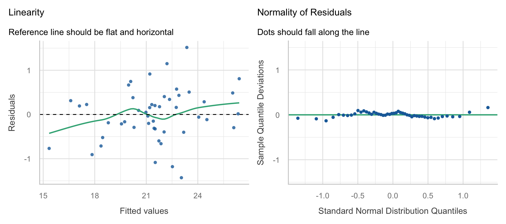
Look for patterns and changing spread in unexplained differences against fitted values, and departures from the reference line in the other panel. A reassuring plot does not establish adequate washout. Two periods do not provide a reliable way to separate all possible lingering effects from current treatment effects. Failing to detect an order difference also does not establish their absence.
Write three sentences giving the B–A estimate and approximate interval, explaining period and cow terms, and stating the washout assumption. Interpret the estimated average intake difference separately from whether it would matter in practice.
Break 14:55–15:10.
Project checkpoint — 15:10–15:35
Use the project launch and your own group’s case. Save your group’s own analysis planbefore fitting the case model. Spend five minutes mapping units, eight naming the question and model, seven on checks and an alternative, and five saving the plan and receiving targeted feedback. Record missing design information without guessing. Different choices can be defensible when linked to the question and design. Do not add calf, cow or time terms to projects without those features.
The plan records the outcome, comparison direction and scale; treatment assignments and shared measurements; proposed outcome distribution and model in words; two checks and an alternative; sources, assistance and next action. Save revisions with reasons. Continue detailed reasoning within the existing follow-up time.
Compare, report and exit — 15:35–16:00
For each study, explain what was randomly assigned, what a row means, and why observations from the same animal share information. Explain the extra scientific requirement of the crossover.
Individually correct both claims: “48 cow-period records mean 48 separately chosen treatment orders” and “including sequence means washout no longer matters.” Complete 10-02 consolidation within 60 minutes after class.