library("DHARMa")
library("see")09-07 · Sketch repeated measurements
Trace gains from the same animal and identify the conditions shared within pens.
Diagnostic report and after-class work
Load the diagnostic packages
Run this block in Posit Cloud before starting the worksheet. If RStudio prompts you to install a missing package, install it and run the block again. You can also install both packages from the Console with install.packages(c("DHARMa", "see")).
Read the study
Researchers assigned Control to one pen and High fibre to another. Each pen housed three animals. The researchers recorded each animal’s daily gain in grams per day at weeks 0, 1, 2 and 3. These are invented teaching data.
library("dplyr")

bridge <- readr::read_csv("data/repeated-measures-bridge.csv")
bridge |> distinct(pen, diet)
# A tibble: 2 × 2
pen diet
<chr> <chr>
1 R1-P01 Control
2 R1-P02 High fibrehead(bridge, 4)# A tibble: 4 × 5
time_week animal pen diet gain_g_day
<dbl> <chr> <chr> <chr> <dbl>
1 0 R1-P01-A1 R1-P01 Control 722.
2 1 R1-P01-A1 R1-P01 Control 715.
3 2 R1-P01-A1 R1-P01 Control 727.
4 3 R1-P01-A1 R1-P01 Control 764.
NoteIdentify the repeated observations
What does each row measure? Which four rows in the displayed sample come from the same animal? What did the researchers assign a diet to?
TipCheck your answer
Each row records one animal’s gain in g/day at one week. The four rows shown are weeks 0–3 for R1-P01-A1. Researchers assigned diets to pens. Every animal in a pen received its pen’s diet.
Sketch three trajectories
The table puts each selected animal’s four gains in its own column. An animal’s trajectory is the sequence of its measurements over time.
Code
bridge |>
  filter(animal %in% c("R1-P01-A1", "R1-P01-A2", "R1-P02-A1")) |>
  select(time_week, animal, gain_g_day) |>
  tidyr::pivot_wider(
    names_from = animal,
    values_from = gain_g_day
  )
# A tibble: 4 × 4
time_week `R1-P01-A1` `R1-P01-A2` `R1-P02-A1`
<dbl> <dbl> <dbl> <dbl>
1 0 722. 679. 720.
2 1 715. 703. 752.
3 2 727. 711. 766.
4 3 764. 727. 773.
NoteDraw and compare the three animals
Put week on the horizontal axis and gain (g/day) on the vertical axis. Plot the four points for each animal and connect that animal’s points. Label the pen and diet for each line. Which two animals share a pen? Find one difference in how their gains change across the four weeks.
TipCheck your sketch
In the plot, find R1-P01-A1 and R1-P01-A2 in the Control pen, and R1-P02-A1 in the High fibre pen. The first Control animal’s gain dips from week 0 to week 1. The second Control animal’s gain rises over that same interval. Each point shows an observed gain and each line joins observations from one animal.
Code
library("ggplot2")

ggplot(
  bridge,
  aes(time_week, gain_g_day, group = animal, colour = animal)
) +
  geom_line() +
  geom_point() +
  facet_wrap(vars(pen, diet), nrow = 1) +
  scale_x_continuous(breaks = 0:3) +
  labs(x = "Time (weeks)", y = "Gain (g/day)", colour = "Animal") +
  guides(colour = guide_legend(nrow = 2, byrow = TRUE)) +
  theme_minimal() +
  theme(legend.position = "bottom")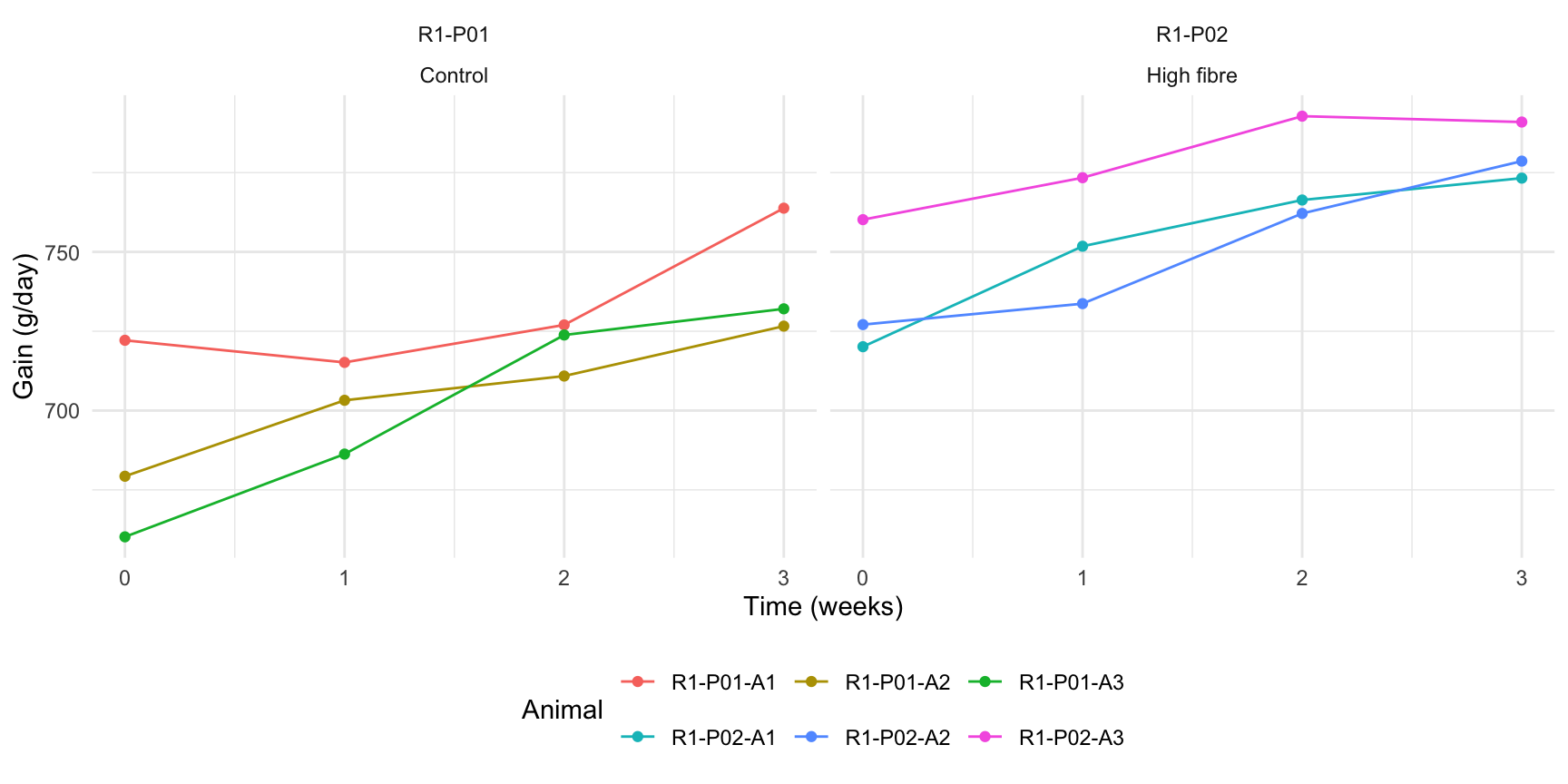
Ask what the design can tell you
NoteInterpret the trajectories
Write a question about whether the diet difference changes over time. Why might two gains measured a week apart on the same animal be more alike than gains measured three weeks apart, even after allowing for that animal’s usual gain? Could differences between these two pens be attributed to diet alone?
TipRead an example answer
One question is whether the difference in average gain between diets is larger at week 3 than at week 0. Measurements close together may reflect the same short-term health or feeding conditions for an animal. The plot shows how gains changed in these two pens. With one pen on each diet, any difference between the pens could reflect diet or other conditions shared within each pen.
Bring your sketch, diagnostic report and one question about similarity through time to Class 10.