Case 3 · Starting weight and growth

Check a straight-line relationship and decide whether to fit a curve.

Use this page in class or as a reference later. Complete each formula in your R console or write it down before revealing the solution. Use the displayed output to answer the interpretation questions before checking your answers. To run the analysis, start from the supplied Posit Cloud project root and work through the R blocks in order. If you have yet to fit a model yourself, run the fit in its solution callout before using it in the next block.

Load the diagnostic packages

Run this block in Posit Cloud before starting the worksheet. If RStudio prompts you to install a missing package, install it and run the block again. You can also install both packages from the Console with install.packages(c("DHARMa", "see")).

library("DHARMa")
library("see")

Read the study and prepare the data

Researchers housed 96 animals individually in four rooms, with 12 animals per diet in each room. They recorded each animal’s starting weight before assigning its diet, then measured daily gain (gain_g_day, in g/day). The column weight_c is starting weight in kg minus 30. The researchers want to compare diets while allowing gain to vary with room and starting weight. These data are invented for teaching.

Set Control and R1 as the reference categories.

library("dplyr")

d <- readr::read_csv("data/case-3.csv")
d <- d |>
  mutate(
    diet = factor(diet, levels = c("Control", "High fibre")),
    room = factor(room, levels = c("R1", "R2", "R3", "R4"))
  )

head(d, 3)

# A tibble: 3 × 5
  room  animal diet       weight_c gain_g_day
  <fct> <chr>  <fct>         <dbl>      <dbl>
1 R1    R1-A01 Control      -0.660       680.
2 R1    R1-A02 High fibre    1.91        754.
3 R1    R1-A03 Control      -7.10        604.

Fit a straight-line relationship

Write the starting formula

Fill both sides of the formula to model gain using diet, room and centred starting weight. What does the weight term assume about the expected change in gain for each additional kilogram of starting weight?

Formula template. Fill in the blanks before running it.

original <- lm(___ ~ ___, data = d)

Check the starting formula

The straight line assumes the same change in expected gain per extra kilogram throughout the observed weight range.

original <- lm(gain_g_day ~ diet + room + weight_c, data = d)

summary(original)


Call:
lm(formula = gain_g_day ~ diet + room + weight_c, data = d)

Residuals:
     Min       1Q   Median       3Q      Max 
-129.374  -30.099    9.106   34.216  110.939 

Coefficients:
               Estimate Std. Error t value Pr(>|t|)    
(Intercept)     677.803     12.296  55.122  < 2e-16 ***
dietHigh fibre   33.661     11.021   3.054  0.00297 ** 
roomR2            2.710     15.588   0.174  0.86239    
roomR3           18.434     15.685   1.175  0.24298    
roomR4           36.478     15.555   2.345  0.02122 *  
weight_c          2.624      1.058   2.481  0.01495 *  
---
Signif. codes:  0 '***' 0.001 '**' 0.01 '*' 0.05 '.' 0.1 ' ' 1

Residual standard error: 53.88 on 90 degrees of freedom
Multiple R-squared:  0.2061,    Adjusted R-squared:  0.162 
F-statistic: 4.673 on 5 and 90 DF,  p-value: 0.0007729

Check residuals against starting weight

A residual is observed minus fitted gain. The QQ plot checks the overall shape of those residuals. The second plot keeps each animal’s starting weight visible.

library("performance")
plot(check_model(original, check = "qq"), n_columns = 1)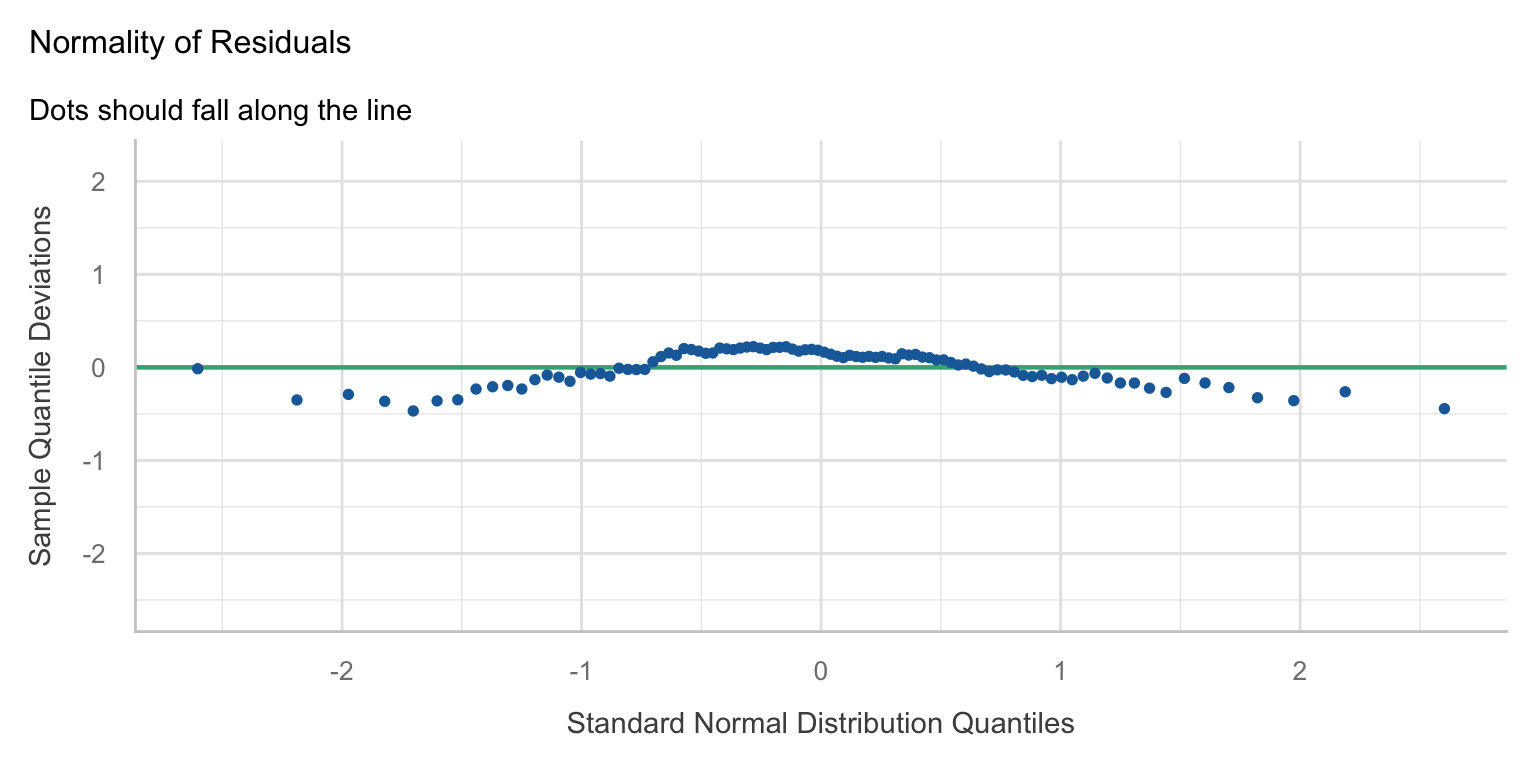

plot(
  d$weight_c,
  residuals(original),
  xlab = "Starting weight minus 30 kg",
  ylab = "Observed minus fitted gain (g/day)"
)
abline(h = 0, lty = 2)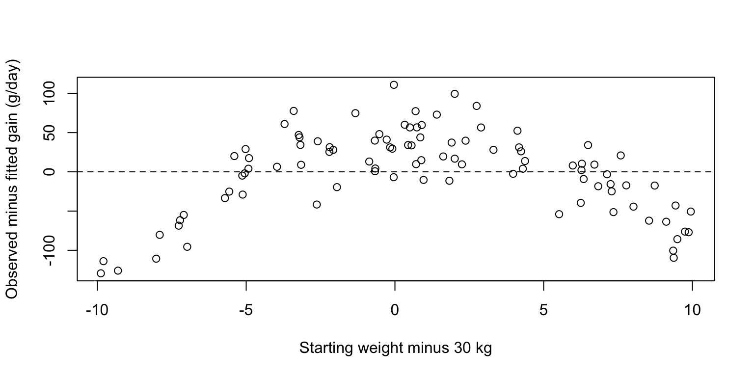

Locate the pattern

Where are residuals mostly above or below zero? Where does the model tend to overpredict gain? Would the QQ plot alone have told you where?

Interpret the weight plot

Residuals are generally higher around intermediate weights and lower at the light and heavy ends. The model tends to underpredict gain in the middle and overpredict it at the ends. The QQ plot combines animals across all weights, so it cannot locate those errors.

Allow the relationship to bend

Complete the curved model

Keep the terms from the first fit and add the square of centred weight. In an R formula, I() tells R to do the arithmetic inside the parentheses. Write the revised formula and predict how the residual plot might change.

Formula template. Fill in the blanks before running it.

revised <- lm(___, data = d)

Check the curved formula

The squared term lets the slope change with starting weight. Keeping the linear term allows the curve to rise or fall at the 30 kg reference weight.

revised <- lm(
  gain_g_day ~ diet + room + weight_c + I(weight_c^2),
  data = d
)

summary(revised)


Call:
lm(formula = gain_g_day ~ diet + room + weight_c + I(weight_c^2), 
    data = d)

Residuals:
    Min      1Q  Median      3Q     Max 
-59.599 -17.446  -0.664  16.056  80.093 

Coefficients:
                Estimate Std. Error t value Pr(>|t|)    
(Intercept)    704.64725    6.32325 111.438  < 2e-16 ***
dietHigh fibre  31.23375    5.48065   5.699 1.54e-07 ***
roomR2          26.82542    7.88413   3.402    0.001 ** 
roomR3          45.71209    7.96874   5.736 1.31e-07 ***
roomR4          56.83927    7.82941   7.260 1.39e-10 ***
weight_c         5.08607    0.54628   9.310 8.55e-15 ***
I(weight_c^2)   -1.59514    0.09616 -16.589  < 2e-16 ***
---
Signif. codes:  0 '***' 0.001 '**' 0.01 '*' 0.05 '.' 0.1 ' ' 1

Residual standard error: 26.78 on 89 degrees of freedom
Multiple R-squared:  0.806, Adjusted R-squared:  0.7929 
F-statistic: 61.62 on 6 and 89 DF,  p-value: < 2.2e-16

plot(
  d$weight_c,
  residuals(revised),
  xlab = "Starting weight minus 30 kg",
  ylab = "Observed minus fitted gain (g/day)"
)
abline(h = 0, lty = 2)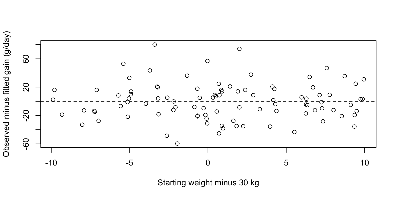

Compare the diets and interpret the curve

The plot shows fitted gains for room R1 across the recorded weight range. The two comparisons below use all recorded animals. For each animal, predict both diets at its recorded room and weight, subtract Control from High fibre, then average the differences with equal weight per animal.

library("marginaleffects")
plot_predictions(revised, condition = c("weight_c", "diet"))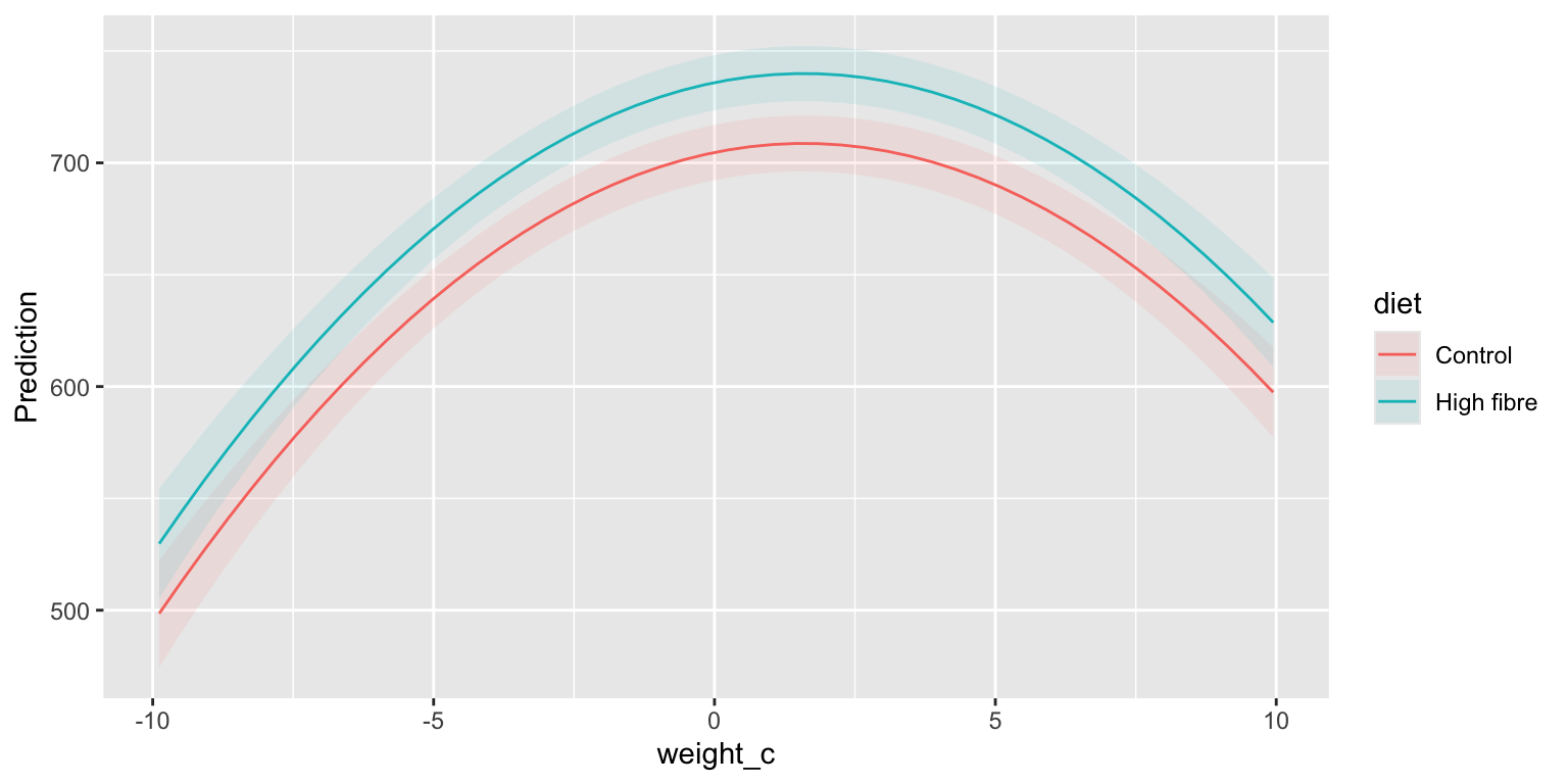

avg_comparisons(original, variables = "diet")


 Estimate Std. Error    z Pr(>|z|)   S 2.5 % 97.5 %
     33.7         11 3.05  0.00226 8.8  12.1   55.3

Term: diet
Type: response
Comparison: High fibre - Control

avg_comparisons(revised, variables = "diet")


 Estimate Std. Error   z Pr(>|z|)    S 2.5 % 97.5 %
     31.2       5.48 5.7   <0.001 26.3  20.5     42

Term: diet
Type: response
Comparison: High fibre - Control

Explain the effect of the change

What happened to the residual pattern? Where do the fitted curves flatten or turn? Read the diet differences and 95% intervals from both models. What would you report, and over which weight range?

Interpret the recheck and diet comparison

The curved pattern in the residuals is much weaker. The predictions rise and then turn down at about 32 kg. Both models estimate higher gain under High fibre. With the curve, the estimated difference is about 31 g/day with a 95% interval of about 20 to 42 g/day, compared with about 34 g/day and an interval of 12 to 55 g/day for the straight line. The curved model better describes the observed starting weights, about 20 to 40 kg. Extending that curve beyond those weights would require further evidence.