Case 2 · Animals sharing pens

Check whether gains from animals in the same pen share a pattern.

Use this page in class or as a reference later. Complete each formula in your R console or write it down before revealing the solution. Use the displayed output to answer the interpretation questions before checking your answers. To run the analysis, start from the supplied Posit Cloud project root and work through the R blocks in order. If you have yet to fit a model yourself, run the fit in its solution callout before using it in the next block.

Load the diagnostic packages

Run this block in Posit Cloud before starting the worksheet. If RStudio prompts you to install a missing package, install it and run the block again. You can also install both packages from the Console with install.packages(c("DHARMa", "see")).

library("DHARMa")
library("see")

Read the study and prepare the data

Researchers assigned Control or High fibre diets to 16 pens in four rooms, with two pens on each diet per room. Six animals shared each pen. Each row gives one animal’s daily gain (gain_g_day, in g/day). The researchers want to compare gain between diets while allowing the rooms to differ. These data are invented for teaching.

Set Control and R1 as the reference categories.

library("dplyr")

d <- readr::read_csv("data/case-2.csv")
d <- d |>
  mutate(
    diet = factor(diet, levels = c("Control", "High fibre")),
    room = factor(room, levels = c("R1", "R2", "R3", "R4")),
    pen = factor(pen)
  )

head(d, 3)

# A tibble: 3 × 5
  room  pen    animal     diet    gain_g_day
  <fct> <fct>  <chr>      <fct>        <dbl>
1 R1    R1-P01 R1-P01-A01 Control       883.
2 R1    R1-P01 R1-P01-A02 Control       819.
3 R1    R1-P01 R1-P01-A03 Control       799.

Fit the starting model

Start with an ordinary linear model. It estimates average gain by diet and room and treats the remaining differences among animals as unrelated.

Write the starting formula

Fill both sides of the formula. Which column is the outcome? Which two terms let the mean differ by diet and room? How many pens received each diet?

Formula template. Fill in the blanks before running it.

original <- lm(___ ~ ___, data = d)

Check the starting formula

Each diet was assigned to eight pens. Each row is an animal measurement, so the dataset contains 48 animals per diet.

original <- lm(gain_g_day ~ diet + room, data = d)

summary(original)


Call:
lm(formula = gain_g_day ~ diet + room, data = d)

Residuals:
     Min       1Q   Median       3Q      Max 
-192.327  -45.290    8.382   50.916  155.732 

Coefficients:
               Estimate Std. Error t value Pr(>|t|)    
(Intercept)      727.17      16.61  43.767  < 2e-16 ***
dietHigh fibre    61.49      14.86   4.138 7.82e-05 ***
roomR2           -22.04      21.02  -1.049   0.2971    
roomR3           -43.75      21.02  -2.082   0.0402 *  
roomR4            99.49      21.02   4.734 8.04e-06 ***
---
Signif. codes:  0 '***' 0.001 '**' 0.01 '*' 0.05 '.' 0.1 ' ' 1

Residual standard error: 72.8 on 91 degrees of freedom
Multiple R-squared:  0.4401,    Adjusted R-squared:  0.4155 
F-statistic: 17.88 on 4 and 91 DF,  p-value: 7.281e-11

Check the gains by pen

A residual is observed minus fitted gain. The QQ plot checks the shape of the residual distribution. In the boxplots, each box groups six residuals from one pen. Look for pens where most animals are on the same side of zero.

library("performance")
library("ggplot2")

plot(check_model(original, check = "qq"), n_columns = 1)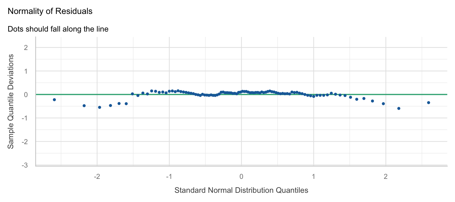

d |>
  mutate(residual = residuals(original)) |>
  ggplot(aes(x = pen, y = residual)) +
  geom_hline(yintercept = 0, linetype = "dashed") +
  geom_boxplot() +
  labs(x = "Pen", y = "Observed minus fitted gain (g/day)") +
  theme_minimal() +
  theme(axis.text.x = element_text(angle = 90, hjust = 1, vjust = 0.5))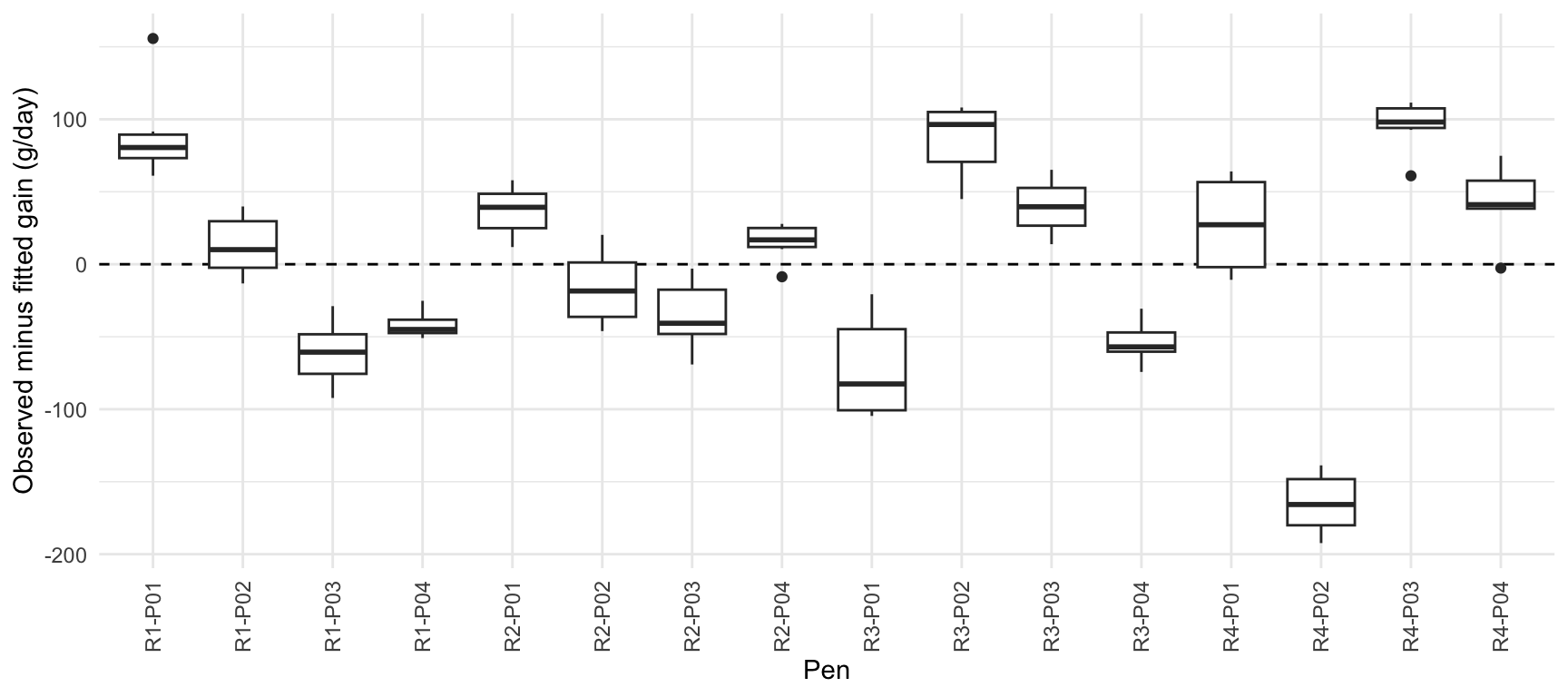

Compare the two plots

Find two pens whose residuals are mostly on opposite sides of zero. What might make gains from animals in one pen similar? Why could a reassuring QQ plot miss that pattern?

Interpret the pen pattern

Several pens have mainly positive or mainly negative residuals. Conditions such as pen temperature or competition for feed could affect the animals sharing a pen. The QQ plot compares the overall residual distribution with a normal distribution. It discards the information about which animals share pens.

Give each pen a shared adjustment

Complete the mixed model

Keep the starting formula and add a random intercept for pen. A random intercept is a shift in expected gain shared by all animals in that pen. Write the term using the form (1 | grouping_variable). What is estimated from the 16 pens?

Formula template. Fill in the blanks before running it.

revised <- lme4::lmer(___, data = d, REML = TRUE)

Check the mixed model formula

The model estimates the spread of pen shifts and the remaining variation among animals. It uses restricted maximum likelihood (REML) to estimate those two sources of variation.

revised <- lme4::lmer(
  gain_g_day ~ diet + room + (1 | pen),
  data = d,
  REML = TRUE
)

summary(revised)

Linear mixed model fit by REML ['lmerMod']
Formula: gain_g_day ~ diet + room + (1 | pen)
   Data: d

REML criterion at convergence: 898.8

Scaled residuals: 
     Min       1Q   Median       3Q      Max 
-1.85848 -0.70262 -0.08312  0.67220  2.79057 

Random effects:
 Groups   Name        Variance Std.Dev.
 pen      (Intercept) 6516.0   80.72   
 Residual              574.1   23.96   
Number of obs: 96, groups:  pen, 16

Fixed effects:
               Estimate Std. Error t value
(Intercept)      727.17      45.45  15.998
dietHigh fibre    61.49      40.66   1.512
roomR2           -22.04      57.50  -0.383
roomR3           -43.75      57.50  -0.761
roomR4            99.49      57.50   1.730

Correlation of Fixed Effects:
            (Intr) dtHghf roomR2 roomR3
dietHighfbr -0.447                     
roomR2      -0.632  0.000              
roomR3      -0.632  0.000  0.500       
roomR4      -0.632  0.000  0.500  0.500

check_convergence(revised)

[1] TRUE
attr(,"gradient")
[1] 1.940595e-08

check_singularity(revised)

[1] FALSE

The residuals below use fitted gains that include each pen’s fitted shift.

d |>
  mutate(residual = residuals(revised)) |>
  ggplot(aes(x = pen, y = residual)) +
  geom_hline(yintercept = 0, linetype = "dashed") +
  geom_boxplot() +
  labs(x = "Pen", y = "Observed minus fitted gain (g/day)") +
  theme_minimal() +
  theme(axis.text.x = element_text(angle = 90, hjust = 1, vjust = 0.5))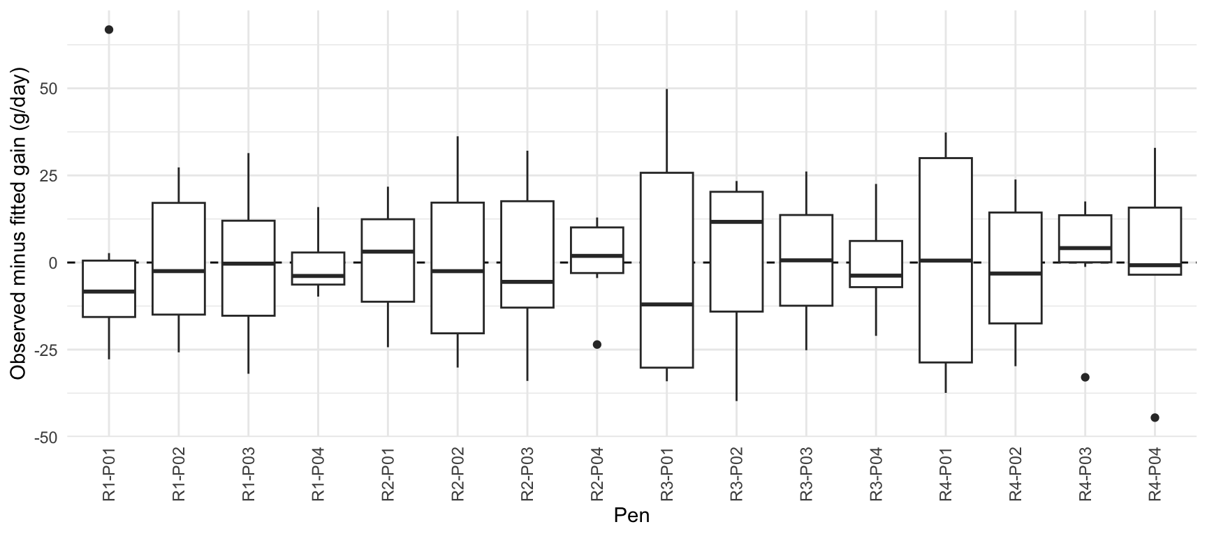

Compare the diet differences

Predict both diets at each animal’s recorded room, subtract Control from High fibre and give each animal equal weight. Every room contributes equally here. For the mixed model, re.form = NA sets the pen shift to zero in both predictions.

library("marginaleffects")
avg_comparisons(original, variables = "diet")


 Estimate Std. Error    z Pr(>|z|)    S 2.5 % 97.5 %
     61.5       14.9 4.14   <0.001 14.8  32.4   90.6

Term: diet
Type: response
Comparison: High fibre - Control

avg_comparisons(revised, variables = "diet", re.form = NA)


 Estimate Std. Error    z Pr(>|z|)   S 2.5 % 97.5 %
     61.5       40.7 1.51     0.13 2.9 -18.2    141

Term: diet
Type: response
Comparison: High fibre - Control

Explain what changed

Compare the residual boxes before and after the change. Find the diet estimate and both 95% intervals. Why can the estimate stay the same while the interval changes? Which result would you report?

Interpret the recheck and diet comparison

The boxes sit closer to zero after the fit includes the shared pen shifts. Both fits estimate about 61.5 g/day higher gain under High fibre. The equal allocation of diets within rooms and equal numbers of animals per pen preserve the estimate here. The interval widens from about 32 to 91 g/day to about −18 to 141 g/day because the analysis accounts for the animals sharing each pen. Report the mixed model estimate and its approximate interval. With 16 pens and no small-sample adjustment, interpret the interval with care.