08-01 · Split plots, Latin squares and unequal groups
Foundations slides · Workshop slides · Student script
Start here
28 October 2026, 12:30–16:00. Open student-starter.R in the supplied 08-glmm-analysis Posit Cloud project. Run its sections in order. Each section shows the package calls directly; there is no analysis helper to load. Required packages are readr, dplyr, tidyr, tibble, lme4, performance, marginaleffects and ggplot2; see draws the check plots. Run setup.R only if packages need installing.
Work in groups of three: one person runs code, one explains the output, and one checks the design. Change roles at 13:55 and 15:10. Use the printed reference output if computing is unavailable. All data are invented teaching examples.
12:30–12:40 · Opening recall
Diet was assigned to sixteen pens, four in each of four rooms. Six animals in each pen were measured once. Draw room → pen → animal. Mark where diet was assigned. Researchers choose a diet separately for each pen, giving eight pens on each diet. All six pigs in a pen eat that pen’s diet. Explain what six more measurements per pen would add, and what they would not add.
12:40–13:20 · Random effects and formula notation
After allowing for diet and room, animals in the same pen may still share conditions. Think of a measured gain as the diet-and-room mean, plus a shared pen difference, plus a remaining animal difference. A random effect describes group differences using a common distribution: here a bell-shaped distribution centred on zero, with its spread estimated from the pens. This describes variation; it does not mean that treatments were randomly assigned.
Read gain_g_day ~ diet + room + (1 | pen) in words. Diet and differences among these four rooms are fixed effects. The term (1 | pen) adds a shared difference for each pen. The 1 means the overall level, or intercept; it does not mean one gram. Read | as “for each group identified by”, and pen as the grouping column. R includes an overall intercept automatically: ~ diet + room means ~ 1 + diet + room. The 1 inside (1 | pen) adds shared pen differences, rather than replacing that overall intercept. A model with both kinds of effects is called a mixed model.
Before fitting, run the pig plot in student-starter.R. Each point is one pig; pens are on the horizontal axis and daily gain in g/day is on the vertical axis. Rooms have separate panels and colour identifies diet. Horizontal jitter separates overlapping points without changing their gains. Compare pigs within one pen, then pens within the same room.
Fit the Gaussian shared-pen model with lme4::lmer() and REML = TRUE. Read the complete summary. The other Gaussian mixed models also use lme4::lmer() with REML; models without random effects use lm().
Run the first section of student-starter.R through the ranef() and VarCorr() output. Read four fitted pen differences in grams/day. A positive value places that pen above its diet-and-room expectation. These are partly pooled estimates: with limited information, a pen’s estimated difference is pulled towards zero. VarCorr() gives the estimated spread among pens and the remaining spread among animals. The centre of the assumed distribution is zero; fitted pen values need not average to exactly zero.
Run random-effects-plots.R separately. Its forty calf mean lines are illustrations specified from invented values, not fitted results or observed weights. The intercept-only and varying-slope plots use the same starting differences and weight scale. Weekly-gain differences now have SD 0.9 kg/week, twice their previous spread, so the slopes vary more visibly. The dashed line is the assumed overall mean; the forty drawn lines need not average exactly onto it.
In weight_kg ~ week + (1 | calf), each calf can have a different starting weight but all have the same weekly gain, so lines are parallel. In weight_kg ~ week + (1 + week | calf), week outside the brackets describes average weekly gain, and week inside allows each calf to differ from it. A slope is change in weight per week. The notation also allows starting and gain differences to be related; the original illustration draws each calf’s starting and gain differences separately, using the same distributions for every calf.
Centre time by calculating week_c = week - 4. The new intercept is the calf’s mean weight at week 4. Keep the same weight paths by changing the fixed intercept to 42.2 kg and the calf’s intercept difference to its original starting difference plus four times its gain difference. The printed maximum path difference is only computer rounding. The weekly gains do not change. Starting and gain differences can become related after this change of origin; centring does not guarantee that they become unrelated.
Explain why different calf slopes need repeated measurements at different weeks. Each pen receives one diet, so (1 + diet | pen) would ask for pen-specific diet changes unsupported by this study. Save the comparison with a model that ignores pens and its numerical checks for the existing after-class review.
13:20–13:40 · Split plots
In a new experiment, each pen is divided into two fenced sections. The whole pen receives one diet. For each pen, researchers randomly choose whether its Left or Right section gets deep bedding; they put standard bedding in the other section. Assume bedding does not move between sections. Measure one average gain for each section.
See the one-pen sketch and four-room sketch. Both bedding sections in a pen receive the same diet; the fence keeps pigs and bedding separated.
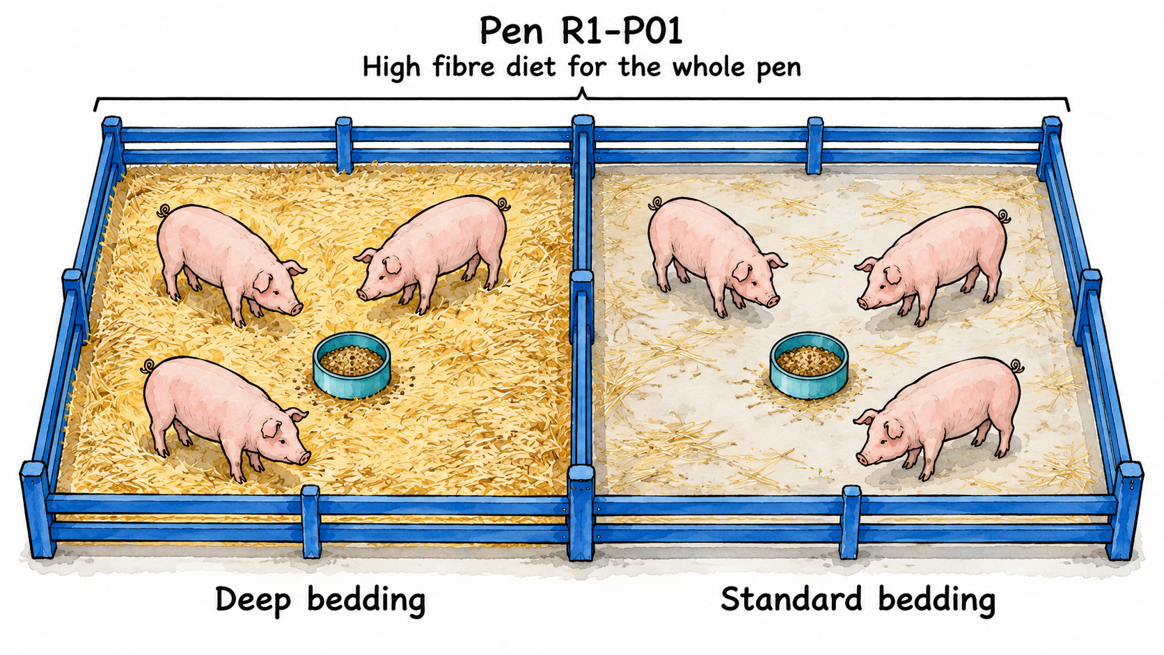
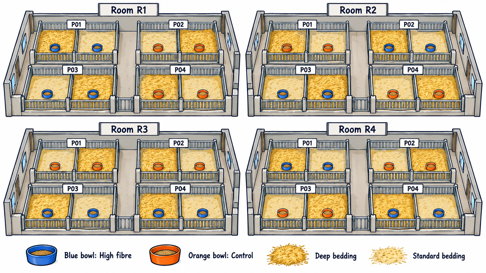
Run section 2 and sketch two pens. Label diet on each pen and bedding on each section. A split-plot design assigns different treatments to different sizes of unit. We have sixteen pens and 32 section averages; we do not have 32 independent diet assignments.
diet * bedding lets the diet difference change with bedding. This changing difference is called an interaction. Explain why the model includes a shared pen difference even though each row now represents a section.
Using newdata = "balanced" gives each room equal weight within every diet and bedding combination. re.form = NA leaves out differences fitted for particular existing pens. In this continuous Gaussian example, this also gives the mean over the assumed zero-mean pen differences.
Use avg_comparisons() for High fibre minus Control within each bedding. Compare Deep minus Standard within each diet during the after-class review. For one row, write a sentence naming direction, units, estimate and uncertainty. Describe what further evidence would be needed before claiming a changing treatment difference.
Break 13:40–13:55.
13:55–14:25 · Latin squares
Sixteen broiler pens occupy four rows and four columns. Light differs between rows and airflow between columns. Each pen receives one feed, A–D, throughout the trial; each feed occurs once in every row and column. Pens have equal numbers of birds of the same age. Record one mean daily gain per pen in grams per bird per day over the same trial period. Feed stays within its assigned pen. This spatial layout is a Latin square; there are no feed changes or repeated periods.
Run section 3 using broiler-latin-square.csv. Draw the allocation and locate all four pens receiving feed A. Explain the row and column tables. Randomly choose row order, column order and feed labels of a valid square before the trial, then record those choices.
Use lm() to adjust for these four rows and columns as fixed effects; one pen mean per record needs no shared pen term. The model assumes that feed, row and column differences add together. Interpret C minus A from avg_comparisons(), including its units and interval. Each pen counts equally; this additive contrast is the same at every position. The t interval uses six error degrees of freedom and assumes independent normal errors with common variance. One small square does not establish those assumptions.
Suppose C works differently in every row. Explain why one pen per position cannot separately estimate every feed-by-row change, every feed-by-column change and ordinary pen variation. More birds in the same pens do not add feed assignments. More model terms cannot create missing replication.
The original greenhouse fertiliser example is retained in the workshop’s backup slides for future Agroecology cohorts, using latin-square.csv.
14:25–14:55 · Unequal group sizes
An equipment fault loses both section averages from R1-P01 and the Left section of R3-P02. In this hypothetical example the fault is unrelated to growth. Run section 4.
Count the original sixteen assignments separately from the fifteen pens still represented. Check counts by room, diet and bedding. Unequal counts can also be planned, for example because a treatment is costly; they are a property across designs, rather than a replacement for identifying the treatment assignments.
Compare raw observed means with model-adjusted means giving every room equal weight. Explain which question each table answers. Use newdata = "balanced" and re.form = NA for both complete and unequal data, so every room keeps equal weight and fitted pen differences are excluded. The model does not reconstruct the missing observations.
Would this be credible if slow-growing animals were more likely to disappear? Write the missing information you would request. Would all treatment comparisons remain available if an entire treatment combination had never been observed? Explain why accepting unequal counts is not a cure for all missing-data problems.
Break 14:55–15:10.
15:10–15:30 · Gaussian calf differences and a model check
Recall the forty simulated calf paths: overall starting weight 35 kg and weekly gain 1.8 kg/week. Each calf has a starting-weight random effect and a weekly-gain random effect. The simulation uses a starting-weight distribution with mean zero and SD 4 kg for every calf, and a weekly-gain distribution with mean zero and SD 0.9 kg/week. We draw each calf’s pair without using the other calves’ draws. The pairs are independent and identically distributed (i.i.d.) across calves. Gaussian means normal. The two components have different units and spreads; “identically distributed” applies to the same pair distribution being used for every calf.
Open reference/random-effects-normal-qq.png, or run the plotting script to produce it. Each panel compares forty simulated calf random effects with a normal reference. Starting-weight effects stay in kg and weekly-gain effects in kg/week; each panel has its own vertical scale. The dashed line matches a normal shape to the sample quartiles. We are illustrating distributional shape, rather than comparing coefficients or changing the scale of a treatment effect. avg_predictions() and avg_comparisons() answer questions about expected outcomes and contrasts; they do not replace a distributional check. We generated the values from that model, so this illustrates an assumption rather than checking a real study. A QQ plot also cannot tell us whether real calves share a feeder or disease outbreak. Recorded weights from one calf share its calf differences; they are not separate i.i.d. observations.
After centring, weight and gain differences within a calf can be related while the pairs still follow the same Gaussian distribution across calves. The standard random-slope formula allows that relationship. Fitted, partly pooled pen differences should not be treated as raw draws like the values in this illustration.
Recall the complete split-plot pig study using the one-pen and four-room images. Diet goes to whole pens, bedding to fenced sections; there are 32 section means from sixteen pens. Check split_fit, fitted to the complete study. In the residual-versus-fitted plot, describe whether the green line is roughly horizontal near zero or has a clear curve. Would that pattern prompt further investigation of the mean model? Next, inspect a normal QQ plot of section residuals: do points follow the line through the middle and at both ends? Finally, use check_predictions() to compare observed gains with 50 model-simulated datasets, drawing new pen effects with re_formula = NA. Compare centre, spread and tails. State one feature the model captures well or poorly. These plots cannot establish randomisation or physical separation of bedding.
15:30–15:45 · Project design and data audit
Draw the design for your own study. Record treatment assignment or sampling, independent units, shared groups, repeated measurements, unequal counts and unknown information. Name the data source and next action before 4 November. Keep source-paper facts separate from the teaching simulations. Observational studies require association wording rather than a treatment claim.
15:45–16:00 · Exit and follow-up
Explain why assigning diet to pens and bedding to sections is split plot, and why losing a section also makes the recorded data unbalanced. Explain what more animals would change.
Save your script, annotated output and diagram. Complete the after-class handout in 75 minutes. Use the final task to try larger pen counts and recommend a plan with at least 0.8 power.